RAHUL LESLIE'S BLOG POSTS:-
Time History input file generator for ANSYS Classic
This application program, or app, converts the earthquake data in Excel (or in text file form), such as, for example:
|
TIME. |
ACCEL. |
|
0 |
0.00778 |
|
0.02 |
0.01687 |
|
0.04 |
0.01835 |
|
0.06 |
-0.04036 |
|
0.08 |
-0.00771 |
|
0.1 |
-0.02079 |
|
0.12 |
-0.01367 |
|
0.14 |
-0.02922 |
|
0.16 |
-0.08288 |
|
… |
… |
for Time History analysis, to an input format file for ANSYS Classic. This is primarily because the method of inputting data for Time History is cumbersome, having to write a loop using APDL script that reads in the data file. It becomes even more complicated for multiple sets of nodes with different Time History data. This app is made to ease the effort...
...by
writing out those different load-steps, not as a loop, but listing out the
complete loading steps one after another into a MAC file, which can then be
read into ANSYS to run the time history analysis.
This app, as of now is developed for the
time-integration approach implementing the default method (ie., Newmark method
in present versions of ANSYS). However, the default method works fine (and
fast) with linear analysis models too.
The
input data for the app is provided through the Excel sheet provided (in the
column ‘U’), as shown below

The contents of the Excel sheet and the data to be
filled in are as follows (see fig. above – the sheet named ‘Data’). Please note
that parameters are meant to be entered only in the yellow-coloured cells.
- No of sets:
In this app up to three sets of data can be input. For seismic analysis
(by base excitation, usually only one set is required – all supported nodes
are excited with the same earthquake record. The entry for such cases is
‘1’
In case loads are applied at
multiple points, for example, in off-shore structures, there can be, say, three
sets of nodes, each to be applied with a different force time-history values, a
value of, 2, or 3, can be entered, as the case might be.
Also, in case of base
excitation seismic analysis, where the X, Y and Z components of the earthquake
record are simultaneously being applied on the structure, a value of 3 is to be
entered.
- Scale factor:
If the input values of data record is to be scaled to some factor, for example, if an earthquake record in terms of ‘g’, then the conversion scale factor of 9.81
(depending on the units used) is to be entered to convert it to absolute
units. Also, if, for example, a force-vs-time values are provided in kN,
whereas the ANSYS model is being done in N, then the conversion factor of
1000 should be entered. If no conversion is to be done, a value of ‘1’
should be entered. In a nutshell, the values of data will be multiplied by
the scale factor before application of the structure.
- Time values from file: If time is not is not listed against the data in
the time history record, but specified as being in constant intervals, ‘N’
should be entered, and input the constant time interval for which the time
history data is given in entry no. 4.
- Time Intervals: For cases where the entry in no. 4 is ‘N’, the constant time interval for which the time history data is given in entered. Time is entered in the MAC file using the APDL command of TIME
- Output File Name: It is the name of the file to be generated by the app. It may be
same as that of ANSYS model file. The name of the file generated will be
the name entered, but with the extension “.MAC”
- Input data type:
Time History Analysis can be done for
a. nodal (ground) displacement (enter D),
b. nodal velocity (enter V),
c. nodal (ground) acceleration (enter A),
d. body acceleration (enter B), and
e. nodal forces (enter F)
The alphabets given in the
brackets corresponding to the type of analysis to be done is to be entered.
Except for body acceleration, all other types need list of nodes, and up to
three sets of data can be provided.
The data is entered in the MAC
file, for entries corresponding to (a) to (e) above using the APDL commands
of (a) D,..UX, (b) D,..VELX,
(c) D,..ACCX, (d) ACEL
and (e) F,..FX respectively (listed
here with samples for X direction)
- Direction of application: Direction of application of data can be along
global X, Y or Z. It can be different for each set of data.
- Should substeps specification be given in terms of duration/substep?
(Y/N): If time data is read from file, and time
intervals are not constant, it might be more appropriate to adjust the no.
of sub-steps to match time steps. To do this, enter ‘Y’. All the instructions
shown in blue in the picture (of the picture of the Excel sheet above)
shown above disappears when ‘N’ is entered instead.
- Should min. substeps alone be given in terms of no. of substeps?
(Y/N): Even with the
input option switched to duration/sub-step, the min. Sub-steps can still
be chosen to be given as no. of sub-steps itself. The instruction shown in
green in the picture (of the Excel sheet) shown above disappears when ‘N’
is entered
- Duration/substep in each time step: The values of sub-step duration provided subsequently should be calculated and provided. For example, if the time interval is 0.02 sec, and you intend to give 4 sub-steps, then enter value of 0.005 (= 0.02 / 4). The program will then automatically adjust the no. of subsets for subsequent load steps – if, for example, time interval is 0.06 sec., no. of sub-steps will automatically set as 12 (= 0.06 / 0.005), and if it is 0.01 sec., no. of sub-steps will be 2 (= 0.01 / 0.005). Enter for all three parameters, such that duration for min. Sub-steps > duration for nominal Sub-steps > duration for max. Sub-steps.
- Min. no. of steps: If the entry to 9 above is ‘Y’ then the min. No. of sub-steps should be entered. This is to prevent the min. no. of sub-steps to be neither just 1, nor a high value, in due of the calculations. Putting this to a bare minimum (say, 2 or 3 will help in faster completion of analysis.
- Duration/substep in each time step: Enter the nominal steps, max. no. Sub-steps and min. no. of steps. Note: min. no. of Sub-steps < nominal no. of steps < max. no. of Sub-steps. The three substep parameters are entered in the MAC file using the APDL command of NSUBST
- Does the model have SOLID65 or use Element Birth/Death feature?
(Y/N): Earlier versions of ANSYS did not allow
use of LSWRITE and LSSOLVE commands with models containing Element
Birth/Death feature or SOLID65 (Concrete element), in which, one had to
proceed with multiple SOLVE commands. That’s why the program asks this, on
order to put commands in the ANSYS input file appropriately.
- Should results of all sub-steps be written? (Y/N): The analysis saves results for all
the sub-steps, if ‘Y’ is entered. Otherwise only the last sub-step of
every load-step is saved, an option of ‘N’ selected usually when disk space
is low.
- Include damping? (Y/N): Enter ‘Y’ to include damping ratio.
- Damping ratio: Damping value can be entered either
as Constant (using DMPRAT command in ANSYS), or as per option
provided in entry no. 17 below. Here, the damping ratio, in percentage is
to be entered. Eg, if damping is 3%, enter 3 (not 0.03).
- Include alpha & beta instead of Const damping: Damping value can be entered either as
Constant (in entry no. 16 above), or with proportionate damping (using ALPHAD
and BETAD commands in ANSYS). Enter ‘Y’ for proportionate damping.
- Frequency: When ‘Y’ is provided for entry no. 17 above, the
modal frequency of the structure should be entered.
The values vs time data are to be provided in the ‘Data’
sheet itself as seen below

The first, second and third set of data are to be
pasted in the columns B, C, and D respectively (marked B, C and D in red),
leaving out the first row for heading. If only one set of data is to be
provided, use only the B column (marked B in red). If time data is also
provided, paste it in the A column (marked A in red), of course, leaving out
the first row for heading. If time is to be provided as fixed intervals, then
it is not required to provide anything in the A column. As such, the no of data in all the
four columns provided with data are expected to be of equal numbers. During the pasting of data, if from another Excel
file, it might have the Excel sheet cells lose their colour seen above in
picture, but that is okay, and no way affects its working.
Except
for Body Force data, all other data requires list of nodes to apply the load
to. It is to be provided in the ‘NodePt’ sheet as seen below

For example, for base excitation, acceleration values are to applied to all the support points, for which the list of all the support node numbers are to be provided. The first, second and third set of node lists are to be pasted in the columns A, B, and C respectively (marked E, F and G in red), leaving out the first row for heading. If only one set of data is to be provided, correspondingly, only one set of nodes are to be provided, and use only the A column (marked E in red). Each sets of nodes might have a different number of nodes, as the case may be.
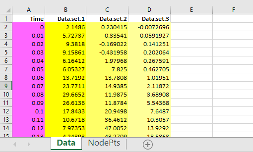
For
example, in off-shore structures, there can be, say, three sets of nodes, each
to be applied with a different force time-history values, as say, listed below:
The number of data in the force vs. time tabulation should be the same, and the
time (if provided) should also be same and common…
|
TIME. |
FORCE ON NODE SET 1 |
FORCE ON NODE SET 2 |
FORCE ON NODE SET 3 |
|
0 |
2.1486 |
0.230415 |
-0.0072696 |
|
0.01 |
5.72737 |
0.33541 |
0.0591927 |
|
0.02 |
9.3818 |
-0.169022 |
0.141251 |
|
0.03 |
9.15861 |
-0.431958 |
0.202064 |
|
0.04 |
6.16412 |
1.97968 |
0.267591 |
|
0.05 |
6.05327 |
7.825 |
0.462705 |
|
0.06 |
13.7192 |
13.7808 |
1.01951 |
|
0.07 |
23.7711 |
14.9385 |
2.11872 |
|
0.08 |
29.6652 |
11.9875 |
3.68908 |
|
0.09 |
26.6136 |
11.8784 |
5.54368 |
|
0.1 |
17.8433 |
20.9498 |
7.6487 |
|
0.11 |
10.6718 |
36.4612 |
10.3057 |
|
0.12 |
7.97353 |
47.0052 |
13.9292 |
|
0.13 |
4.24393 |
43.2709 |
18.5863 |
|
… |
… |
… |
… |
… and say, the 1st set of nodes contain 5
nodes, the 2nd set contains 3 nodes and the 3rd set
contains 2 nodes, as shown below:
The node numbers of all the nodes pertaining to the first
set of time varying forces are
437
438
439
440
441
Similarly, the nodes pertaining to the second set of
time varying forces are
746
923
988
and for the third set are
341
647
Then the data entries
in the Excel sheets are to be as shown below:

If seismic analysis is meant to be done with data in all three directions, provide the three components in columns B, C and D in the ‘Data’ sheet, and provide the same set of support node list in the columns A, B and C in the ‘NodePts’ sheet.

After entering the required parameters and data into the Excel sheet, press the ‘Write data files’ button embedded in the ‘Data’ sheet (See the first figure in this page), which then creates the files (1) ‘Para.txt’ file, (2) ‘Data01.txt’, ‘Data02.txt’ and ‘Data03.txt’ files, and (3) ‘Node01.txt’, ‘Node02.txt’ and ‘Node03.txt’ files.
Read this ‘.mac’ file into ANSYS APDL via the menu ‘File > Read input from...’ option, which then starts the Time History analysis process.
2. The Mac Generator
(THGen-Ver-1-02.exe)**
Rahul Leslie
rahul.leslie@gmail.com
May 2021
* https://www.dropbox.com/s/0s4k8m4h1dutkoz/THDat-Ver-1-02-Excel.zip?dl=0
** https://www.dropbox.com/s/gd8nybblxhis5y7/THGen-Ver-1-02-Exe.zip?dl=0